Pythonによる振幅スペクトルと位相スペクトル
目次
概観
フーリエ変換は扱う信号とデータの長さによって四種類あります。
scipy - Fourier Transforms にもある通り、有限長のデータを扱う、離散系でのフーリエ変換(DFT)が実装されています。よくあるライブラリではDFTが実装されていると思います。
今回はPythonを利用してFFTから、振幅スペクトルと位相スペクトルを求めたいと思います。 どのFFTを用いるかとういと、 scipy.fft のFFTを利用します。 scipy.fftpack は利用していません。
一般に無限長のデジタルデータや有限長の連続デジタルデータ(笑)は扱えないので積分記号や無限大記号が入ったフーリエ変換は基本的にライブラリでは実装されていないと思います。
パワースペクトルやパワスペクトル密度を求める際の足掛かりとして振幅スペクトルを正しく表示できる必要があると思います。(パワースペクトルやスペクトル密度に関しては別記事にて書く予定です。)
また、本記事では振幅スペクトルと書きましたが厳密には複素フーリエ係数をスペクトル表現しております。
準備
pipを利用してインストールします。仮想環境を作っておいた方がなにかと良いですよね?!
-
python3(or py) -m pip install numpy
-
python3(or py) -m pip install scipy
-
python3(or py) -m pip install matplotlib
インストールする方法については、 pypa - Installing Packages を参考にしてください!
実装
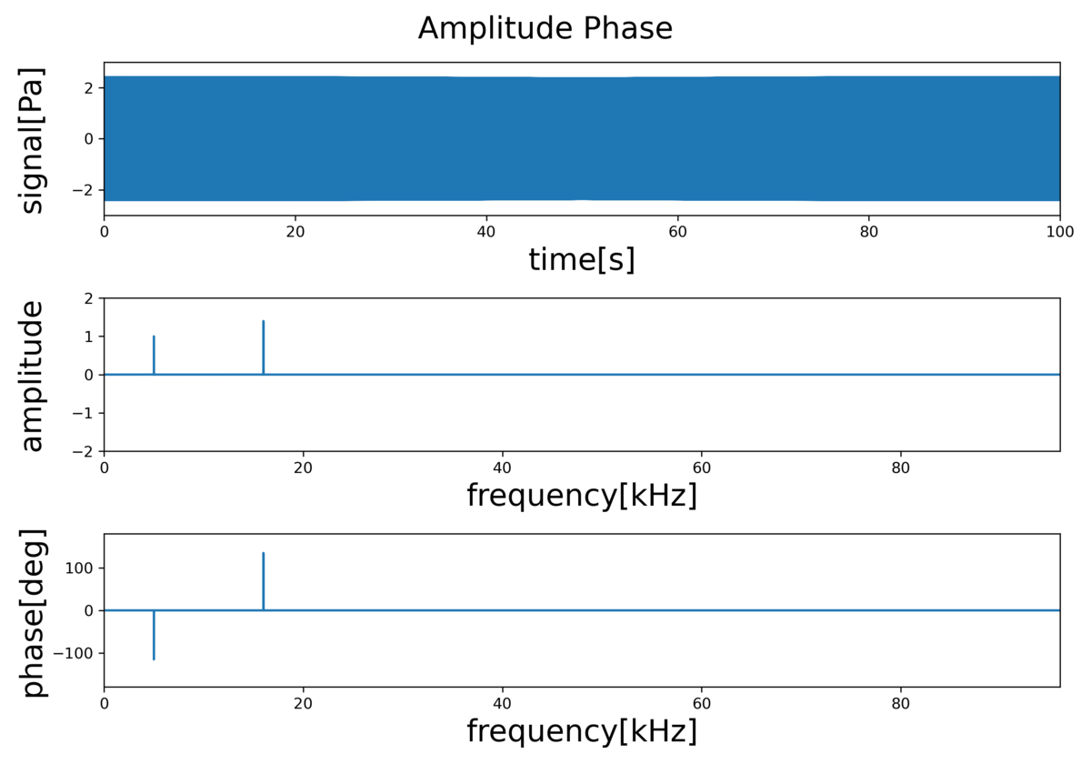
import numpy as np
from scipy.fft import fft, fftfreq
import matplotlib.pyplot as plt

# Defining Constants
T = 100.0
fs = 192.0e3

amp1=1.0
freq1 = 5.0e3
pha1=-2*np.pi/3

amp2=np.sqrt(2.0)
freq2 = 16.0e3
pha2=2*np.pi/3

# Generating Signal
t = np.linspace(0.0, T, int(T*fs))
x = amp1* np.cos(2.0* np.pi* freq1* t+ pha1) \
        + amp2* np.cos(2.0* np.pi* freq2* t+ pha2)

# Doing FFT
fft_signal = fft(x)

# Generating Frequency Vector
f = fftfreq(int(T*fs), 1.0/fs)[0:int(T*fs/2-1.0)]/1.0e3

# Generating Amplitude & Phase
c = np.hstack( \
        ( \
              fft_signal[0] /(T*fs), \
        2.0 * fft_signal[1:int(T*fs/2-1.0)] /(T*fs) \
        ) \
        )
amplitude = np.abs(c)
phase = np.degrees(np.angle(c))
phase = np.where(amplitude < 5e-1, 0, phase)

# Plotting
size_f=20

fig = plt.figure(figsize=[10,7], dpi=300, linewidth=0.0, tight_layout=T)

axs = fig.subplots(3, 1)

ax0 = axs[0]
ax1 = axs[1]
ax2 = axs[2]

ax0.plot(t, x)
ax0.set_xlabel('time[s]', fontsize=size_f)
ax0.set_ylabel('signal[Pa]', fontsize=size_f)
ax0.set_xlim(t[0], t[-1])
ax0.set_ylim(-3, 3)

ax1.plot(f,amplitude)
ax1.set_xlabel('frequency[kHz]' ,fontsize=size_f)
ax1.set_ylabel('amplitude' ,fontsize=size_f)
ax1.set_xlim(f[0], f[-1])
ax1.set_ylim(-2, 2)

ax2.plot(f,phase)
ax2.set_xlabel('frequency[kHz]' ,fontsize=size_f)
ax2.set_ylabel('phase[deg]' ,fontsize=size_f)
ax2.set_xlim(f[0], f[-1])
ax2.set_ylim(-180, 180)

fig.align_ylabels()
fig.suptitle('Amplitude Phase', fontsize=size_f)
fig.savefig('amplitude_phase.png')
結果
解説
scipy - Fourier Transforms にも書いてありますが、正の周波数帯と負の周波数帯には注意してください。 また、配列の長さで割ることも忘れないようにしましょう!
For N even, the elements
contain the positive-frequency terms, and the elements
contain the negative-frequency terms, in order of decreasingly negative frequency.
matplotlib - Align y-labels にも書いてありますが、fig.align_ylabels()でy軸のラベルを揃えることが出来ます!
Align the ylabels of subplots in the same subplot column if label alignment is being done automatically
補足
Fourier Transforms With scipy.fft: Python Signal Processing にも書いてありますが、 scipy.fft と scipy.fftpack では scipy.fft を利用した方が良いみたいです。
Unless you have a good reason to use scipy.fftpack, you should stick with scipy.fft.
Python Plotting With Matplotlib (Guide) にも書いてありますが、 matplotlib.pylab と matplotlib.pyplot では matplotlib.pyplot を利用した方が良いみたいです。
[pylab] still exists for historical reasons, but it is highly advised not to use.
参考
matplotlib - Plotting the coherence of two signals
fig.tight_layout() っていう関数があることを知らなかったです笑笑[訂正] plt.figure()でtight_layout=Tとすれば良いらしいです
scipy - Fourier Transforms (scipy.fft)
scipy.fftを利用したサンプルプログラムを見ることができます!
SPECTRAL AUDIO SIGNAL PROCESSING
理論部分はここを参考に書いていることが多いです。